Variance Reduction in A/B Testing
data-science tutorial Introduction
In this post, we estimate how variance reduction lowers the required sample size in A/B testing experiments. The
theoretical estimates discussed in Part 1 are
verified with empirical testing on real data in Part 2. The code is
written with MetaFlow and the performance is tracked with CometML. This analysis lays the framework for a dashboard
that an experimenter can use to estimate the sample size and covariate synthesis. All code is available here.
Part 1. Theoretical Impact of Variance Reduction
For a confidence level of 95% and a power of 80%, the number of samples needed increases with sample variance
($\sigma^2$) and decreases with the inverse square of the minimal detectable effect ($\delta$):
$ n = 15.7\frac{\sigma^2}{\delta^2}$ (Eq. 1)
This result utilizes distributional assumptions of the null and alternative hypotheses; see appendix for
derivation that draws from the reference section. To reduce the estimated sample size needed, the experimenter
can
reduce $\sigma^2$ or increase
$\delta$. Variance reduction has been well studied, see reference section for examples. Using the CUPED method
[Deng], the original
square root of variance ($\sigma_o$) has a mathematically defined relationship with the CUPED square root of
variance ($\sigma_c$), parameterized by the correlation of the covariate with the target variable ($\rho$):
$ \sigma_c = \sigma_o \sqrt{1-\rho^2}$ (Eq. 2)
For an experiment with and without CUPED, there are two different required sample sizes,
$n_c$ and $n_o$, respectively. A clear way to algebraically express the impact of CUPED on required sample size is to
take the ratio of these. Using Eq. 1 for required sample size and plugging in Eq. 2 gives:
$ \frac{n_c}{n_o} = \frac{15.7(\sigma_c/\delta)^2}{15.7(\sigma_o/\delta)^2} \rightarrow n_c = n_o
\sqrt{1-\rho^2}$ (Eq.3)
Note that as $\rho$ goes to 1, the number of samples required using CUPED reduces.
A related A/B testing measure, the t-statistic, can also be used to demonstrate the effectiveness of CUPED.
This is what
was empirically measured here. In this case, a larger t-statistic is more desirable, where the
t-statistic is
defined as the ratio of the difference between means and the sample standard deviation:
$ t=\frac{\overline{\Delta}}{\sigma} $ (Eq. 4)
Performing a similar operation as above and using Eq. 2 with Eq. 4, the increase in the t-statistic using CUPED
is a function of $\rho$:
$ t_c=\frac{t_o}{ \sqrt{1-\rho^2}} $ (Eq. 5)
A typical threshold for confidence is 95%, equivalent to a t-statistic of 1.96. The x-axis in Figure 1
shows the value of $t_o$. The base case is $\rho$=0 and when $t_o$=1.96, the p-value is 5%. For a smaller
value of the t-statistic and fixed minimum detectable effect, the p-value is not significant - it is >5%.
Employing CUPED, say with a correlation of $\rho$=0.5 (green line), a lower or 'worse' $t_o$ can still lead to
significance.
According to references [Liou (Facebook), Xie (Netflix)], an observed empirical variance reduction of ~40%
implies
$\rho$=0.6 can be achieved in practice. Alternatively, [Li (DoorDash)] proposes CUPAC, which uses Machine
Learning to synthetically create a covariate, and observations imply $\rho$~0.9.
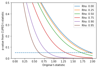
Figure 1: Relationship between t-statistic and p-value. The different lines represents different values of
$\rho$,
the correlation of the covariate to the target variable.
More generally, Figure 2 shows the required correlation for a given t-statistic to get a p-value of 5%.
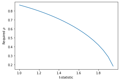
Figure 2: Minimum $\rho$ required for a given value of t in order to get a p-value < 5%.
Part 2. Empirical Confirmation
2.1 Data Description and Modifications
Data was downloaded from the Coveo SIGIR
challenge:
the dataset contains fully anonymized fine-grained events from an online store, i.e. all the products inspected
and purchased by shoppers in a random sample of browsing sessions spanning for several months (the full dataset
contains more than 30M shopping events). Experimentation utilized data from 3/16/2019 to 3/31/2019 as the
treatment and 4/1/2019 to 4/8/2019 as the control. The data was treated as follows. The rows were aggregated by
session_id_hash (a unique identifier of a browsing session by an anonymous shopper) and date and
given a
label
of “1” if any product_action had a ‘purchase’, otherwise it was labeled “0” (that is, all sessions that
led to a
purchase are 1s, sessions without any purchase activity - the majority - are are 0s). The idea is that the
session_id_hash is approximated to the unit of testing and the event of concern is a purchase.
The treatment and control are homogenous because no actual treatment took place. This was confirmed by looking
at the distributional properties of each. The average purchase rate among session ids is ~0.92% with a variance
of 0.0091. There are approximately 44k and 24k sessions in the control and treatment datasets, respectively.
Since no A/B test took place on this data, the binary purchase indicator was artificially modified in the
treatment set.
This is an input that can be varied. For the results below, the treatment target value converts an additional
$\delta$=0.0015 (0.15%) session ids to purchases. This is to simulate the effect of a treatment that
increased purchase rates. This value of $\delta$ calibrates to borderline cases for
detecting effects. The required sample size, using Eq. 1, is approximately 63k, e.g. slightly above the range
used. It also gives a t-statistic of ~1.5 when accounting for both treatment and control variances.
In addition, a covariate was artificially created using a normal random variable and input value of $\rho$ as
follows ($z$ represents the normalized target variable):
$ x = \rho z + \sqrt{1-\rho^2} \ N(0,1) $ (Eq. 6)
2.2 MetaFlow and CometML
The experimental workflow and tracking were done with MetaFlow and
CometML, respectively. First the data is imported, then a covariate
is created using a fixed value of $\rho$, then the treatment is modified. The experiment varied the value of
$\rho$, so that the
foreach function in MetaFlow was used to achieve parallelization. Finally, a p-value
is measured.
The inputs to the experiment are the treatment size and the correlation of the covariate, where the former was set to
$\delta$ =0.0015. For different input values of $\rho$, the t-statistic and p-value are measured so they can be
compared to theoretical results from the previous section.
2.3 Results
Figure 3 shows the t-statistic and p-value as a function of $\rho$ as shown in CometML. In Figure 4, the observed
t-statistic as a function of $\rho$ and plotted against the theoretical value as derived in Eq. 5 indicating
close matching.
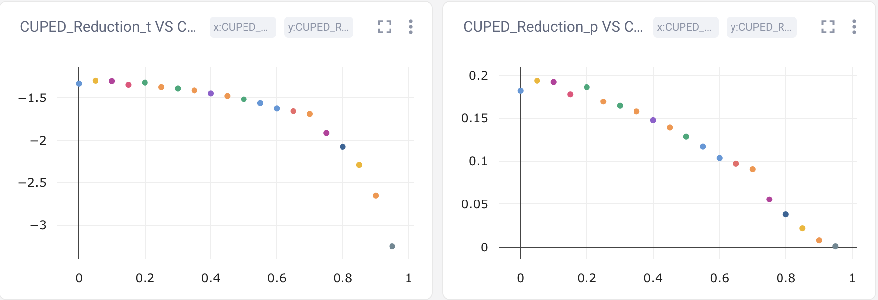
Figure 3: CometML dashboard showing t-statistic (y-axis) vs correlation $\rho$ (x-axis) [left side of figure]
and p-value (y-axis) vs correlation $\rho$ (x-axis) [right side of figure].
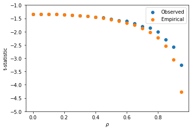
Figure 4: Comparison of theoretical and empirical results (note- ‘observed’ should be ‘theoretical’).
References
- Deng, Xu, Kohavi, Walker. 2013. Improving the Sensitivity of Online Controlled Experiments by Utilizing Pre-Experiment Data.
- Xie, Aurisett. 2016. Improving the Sensitivity of Online Controlled Experiments: Case Studies at Netflix.
- Liou, Taylor. 2020. Variance-Weighted Estimators to Improve Sensitivity in Online Experi- ments.
- Li, Tang, Bauman. 2020. Improving Experimental Power through Control Using Predictions as Covariate (CUPAC).
- Kohavi. 2020. Trustworthy Online Controlled Experiments: A Practical Guide to A/B Testing.
- Dmitriev, Gupta, Kim, Vaz. A Dirty Dozen: Twelve Common Metric Interpretation Pitfalls in Online Controlled Experiments. 2017.
Appendix
Several great explanations exist [see references] that range from extremely technical and non-technical. This section increases the entropy on the topic, but helps convince myself I understand it!
In A/B testing and hypothesis testing in general, there are four potential outcomes:
- Confidence: $P(accept \ H_o|H_o)>1-\alpha$;
- False Positive Rate: $P(reject \ H_o|H_o)<\alpha$;
- Power: $P(reject \ H_o|H_1)>1-\beta$;
- False Negative Rate: $P(accept \ H_o|H_1)>\beta$;
False Positive Rate
To control for the False Positive rate, at a (one-tailed) confidence of 1-$\alpha$, we exploit the law of large
numbers, which allows us to assume that $x_{obs}\frac{\sqrt{n}}{\sigma}$ is standard normally distributed.
Hence, to reject the null hypothesis, we require:
$ P( \ x_{obs}\frac{\sqrt{n}}{\sigma} > \Phi^{-1}(1-\alpha)|H_o \ ) $ (Eq. A1)
Note that using the properties of the normal cdf function, this establishes a FPR of $\alpha$:
$ P( \ x_{obs}\frac{\sqrt{n}}{\sigma}>\Phi^{-1}(1-\alpha)|H_o \ ) =$
$ 1 - P( \ x_{obs}\frac{\sqrt{n}}{\sigma}<\Phi^{-1}(1-\alpha)|H_o \ ) =$
$ 1- \Phi ( \ \Phi^{-1}(1-\alpha) \ ) =$
$ \alpha $
$ 1 - P( \ x_{obs}\frac{\sqrt{n}}{\sigma}<\Phi^{-1}(1-\alpha)|H_o \ ) =$
$ 1- \Phi ( \ \Phi^{-1}(1-\alpha) \ ) =$
$ \alpha $
False Negative Rate
If we assume the null hypothesis ($H_o$) and calculate sufficient confidence, we still cannot rule out the
possibility of a false negative. That is, assuming the alternative hypothesis ($H_1$), we keep $H_o$:
$P(accept \ H_o|H_1)$. To control for this, we would want this probability to be less than a number, $\beta$.
The smaller the $\beta$, the more power ($1-\beta$) the experiment has at reducing False Negatives. We can
write this mathematically by flipping the sign and the conditional in Eq. A1 and requiring that it is smaller
than $\beta$:
$ P( \ x_{obs}\frac{\sqrt{n}}{\sigma}<\Phi^{-1}(1-\alpha)|H_1 \ ) < \beta$ (Eq. A1)
The challenge here is that $x_{obs}\frac{\sqrt{n}}{\sigma}$ is not standard normally distributed, because we
are conditioned on the alternative
distribution, which has a mean shifted away from zero. We can refer to this distance as $\delta$. In
experiments, this is called the minimal detectable effect. The intuition here, is that despite having
an actual mean of $\delta$, the observed sample value (because when we run experiments, we sample from a
distribution) might be some distance away from $\delta$. If this alternative distribution is really wide, then
there’s the possibility that we have enough confidence to keep $H_o$, but insufficient power to reject $H_1$.
To reshape $x_{obs}$ into a standard normal, we shift it by the mean of the alternative distribution by
adding and subtracting $\delta$. Now, $(x_{obs}-\delta) \frac{\sqrt{n}}{\sigma}$ is normally distributed and we
can use cdf mathematics.
$P( \ (x_{obs}-\delta+\delta)\frac{\sqrt{n}}{\sigma} < \Phi^{-1}(1-\alpha)|H_1 \ ) <\beta$
$P( \ (x_{obs}-\delta)\frac{\sqrt{n}}{\sigma} < \Phi^{-1}(1-\alpha)-\delta\frac{\sqrt{n}}{\sigma}|H_1 \ ) <\beta$
$\Phi(\Phi^{-1}(1-\alpha)-\delta\frac{\sqrt{n}}{\sigma})< \beta$
$\Phi^{-1}(1-\alpha)-\delta\frac{\sqrt{n}}{\sigma}< \Phi^{-1}(\beta)$
$\delta\frac{\sqrt{n}}{\sigma}>\Phi^{-1}(1-\alpha)- \Phi^{-1}(\beta)$
$n>( \Phi^{-1} (1-\alpha) - \Phi^{-1} (\beta) )^2 \frac{\sigma^2}{\delta^2} $ (Eq. A3)
Two-Tail Test and Plugging in Values
All of the above assume one-tailed tests. There is a lot of material on whether one should use 1 or 2 tailed tests. Kohavi assumes two-tail, so we modify Eq. A3 to account for this by simply accounting for two sides on the confidence interval:
$n>2( \Phi^{-1} (1-\alpha/2) - \Phi^{-1} (\beta) )^2 \frac{\sigma^2}{\delta^2}$ (Eq. A4)
Plugging in generally accepted values $\alpha$=0.05 and $\beta$=0.20 gets the final estimate of required samples:
$n>2*(1.96+0.84)^2 \frac{\sigma^2}{\delta^2}$
$n>15.7\frac{\sigma^2}{\delta^2}$
$n>15.7\frac{\sigma^2}{\delta^2}$