Linear Regression of Clusters
machine-learning tutorial Introduction
We have all seen a scatter plot that shows a clear linear relationship. I recently came across a financial scatter plot of that appeared to have multiple linear lines describing the data, one for each group of clients (similar to Figure 1 below). Unfortunately, I am not allowed to use that data. So to illustrate a method that automatically fits multiple lines without explicit labeling, I will use the Kaggle Insurance Forecast dataset.
The Data
Figure 1 shows a plot pf dollars charged for a patient versus the age. The plot shows that are possibly three separate linear relationships. Potentially, there can be features beyond age that explain the three groupings. In this case, these features are smoking status and BMI. However, assume your data engineer didn’t track that feature - a common occurrence as the trade-off between tracking every piece of data under the sun can result in unnecessarily burdensome technology stack. How could you discern the underlying behavoir?
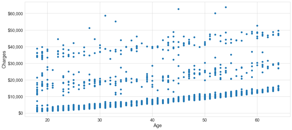
Figure 1
The Model
A mixture model is used to model the relationship between age and charges, by the differeent groups. The user needs to specify the number of clusters/groups (3 groups here). This mixture model can be written as: $F = \pi_1 m_1 + \pi_2 m_2 + \pi_3 m_3$. Here, $\pi_k$ is the probability of a sample being from group $k$, and the prior is modelled as a Dirichlet distribution. Variable $m_k$ is a linear regression model: $m_k= a_k+b_k x$. The generative model is a two-step process, where the overall likelihood of the outcome is minimized:
- Assign each sample in the data to a cluster
- Fit a separate regression line to the set of points assigned to each cluster
$b_1,b_2,b_3 \sim N(10^3, 10^4)$ slope
$\sigma \sim HalfNormal(s =10^4)$ error
The Results
Fitting this yields Figure 2. As you can see, this model fits three lines with their separate intercepts and slopes. In fact, because we know the underlying data, we have the labels. So we can observe in Figure 3 that there is a clear grouping of patients: non-smokers, smokers overweight and smokers non-overweight status.
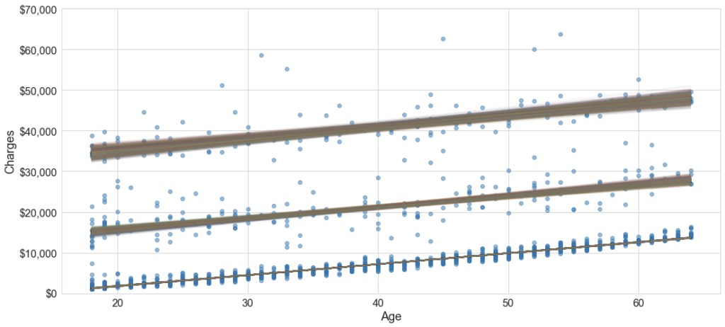
Figure 2
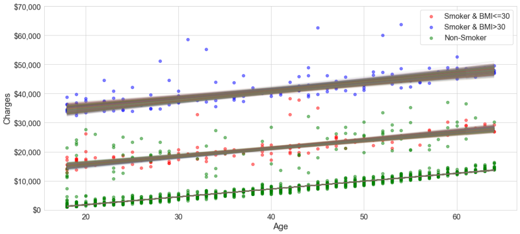
Figure 3
The distributions of the parameters outputted by PyMC3 is presented in Figure 4 (table) and 5 (distribution of slope). Looking at the tabular data in Figure 4, the three line slopes ($\beta_1, \beta_2, \beta_3$) there are two distinct slopes: $269 per year of age for non-smokers and $284 per year age for smokers (both overweight and not). The intercept, which can be interpreted as baseline customer charges is about $19k for smokers, but this number is a bit deceptive. Looking at the marginal distribution of the intercepts (not shown), there are two modes (for both types of non-smokers) around $10k and $30k. The distribution of the population (eg $\pi$) is about 72% non-smokers and an equal 14% of high/low BMI smokers.
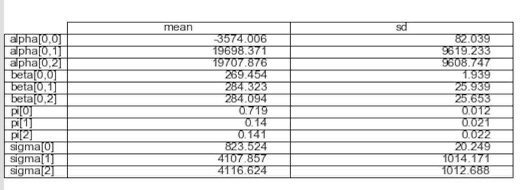
Figure 4
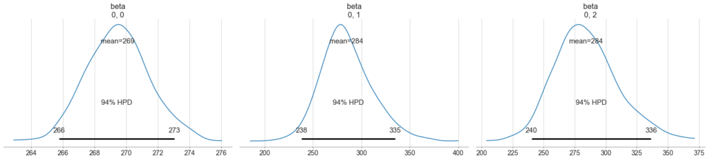
Figure 5
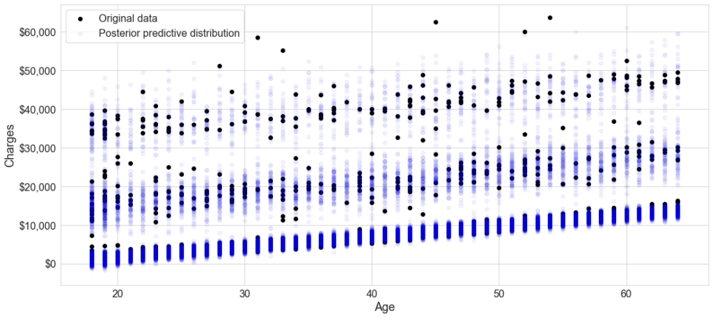
Figure 6